Backpropagation and Gradient Descent: The Backbone of Neural Network Training

Scroll down for Interactive Code Environment 👇

👋 Hi there! In this seventh installment of my Deep Learning Fundamentals Series, lets explore more and finally understand backpropagation and gradient descent. These two concepts are like the dynamic duo that makes neural networks learn and improve, kind of like a brain gaining superpowers! What makes them so mysterious… and how do they work together to make neural networks so powerful?

Neural networks have captivated the world with their remarkable ability to learn and solve complex problems. From image recognition to natural language processing, these powerful models have revolutionized countless industries. But have you ever wondered how neural networks actually learn? What are the mechanisms that allow them to take in raw data, identify patterns, and make accurate predictions?

The key to understanding the learning process of neural networks lies in two fundamental concepts: backpropagation and gradient descent. These two ideas form the backbone of how neural networks adapt and improve over time, continuously refining their internal parameters to minimize the difference between their predictions and the true desired outputs.

In this in-depth blog post, I’ll get under the hood and into the mechanics of backpropagation and gradient descent, exploring how they work together to enable neural networks to learn. I’ll start by breaking down the core principles behind each concept, then see how they are applied in the context of a multi-layer neural network. Along the way, I’ll unpack the mathematical intuitions and dive into real-world code examples to solidify your understanding.

By the end, you’ll have a crystal-clear grasp of the inner workings of neural network training, equipping you with the knowledge to build, train, and refine your own sophisticated models. So, let’s get started and see how backpropagation and gradient descent work!

What is Gradient Descent and Backpropagation?

Think of training a neural network like teaching a student. The network makes predictions, and then backpropagation and gradient descent work together to correct those predictions when they’re off the mark. They do this by adjusting the network’s internal settings, known as weights and biases.

• Backpropagation is like a feedback loop. It calculates how much each weight and bias contributed to the mistake and sends this info back through the network. It’s like saying, “Hey, this setting made us veer off course; let’s adjust it next time.”

• Gradient descent, on the other hand, is the optimizer. It uses the info from backpropagation to adjust the weights and biases, nudging the network towards making better predictions. It’s like a guide that helps the network find the path of least resistance to the right answer.

Together, they form a cycle of continuous improvement. Backpropagation identifies the mistakes, and gradient descent makes the necessary adjustments. It’s a beautiful partnership that refines the neural network’s skills.

Making the Neural Networks Learn

At the heart of neural network training lies the challenge of optimization - how do we find the set of weights and biases that minimizes the difference between the model’s predictions and the true target outputs? This is where gradient descent comes into play, serving as the workhorse algorithm that guides the network towards the global minimum of the loss function.

Imagine you’re standing atop a hilly landscape, and your goal is to find the lowest point as quickly as possible. This is analogous to the optimization problem faced by neural networks - the “landscape” is the loss function, and the “lowest point” represents the configuration of weights and biases that result in the smallest possible error.

Gradient descent works by calculating the gradients, which show the direction of the steepest loss increase. Then, it does the opposite, moving the network towards the global minimum, the optimal solution. It’s like a smart hiker knowing to avoid steep climbs and finding the easiest path down.

The learning rate is like your hiking speed. Too fast, and we might overshoot the minimum and end up unstable. Too slow, and it will take forever to reach your destination. Finding the right balance is crucial for effective learning.

Backpropagation in Action

While gradient descent does the updating, backpropagation provides the directions by calculating the gradients. It’s like backpropagation is the navigator, figuring out the best route by considering past experiences (or, in this case, past predictions).

Despite its name, backpropagation doesn’t involve information flowing backwards. It’s more like a clever use of math, specifically the chain rule in calculus, to efficiently calculate the gradients.

The code starts backpropagation when it begins to calculate the gradient of the loss concerning the final layer’s pre-activation values. This gradient shows how much the loss would change if we tweaked those values.

Then, backpropagation works its way back through the network, layer by layer, using the chain rule to find the gradients for each layer’s weights and biases. It’s like the network is reflecting on how its settings influenced the outcome, and then making informed adjustments.

The key to understanding backpropagation is recognizing that it’s not a mysterious, magical process, but rather a systematic application of the chain rule of calculus. By breaking down the network into its individual layers and components, backpropagation allows us to efficiently compute the gradients required for effective optimization.

Choosing the Right Loss Function

The loss function is the heart of the matter. It measures how well the neural network is doing, showing the difference between predictions and reality. Getting this right is crucial for stable and effective training.

The mean squared error (MSE) loss function is a popular choice. It calculates the average squared difference between predicted and actual outputs, giving us a measure of accuracy. There are other loss functions too, each suited to different types of problems. Choosing the right one is like giving your network the right tools for the job!

What are these Math symbolds?

∂ (Partial Derivative)

In the context of machine learning, specifically within neural networks, differential calculus plays a crucial role. Specifically, the computation of gradients of the loss function with respect to the network’s weights and biases is fundamental. By using partial derivatives, we can compute the gradients needed for updating the weights and biases during optimization. These gradients guide the network to adjust its parameters and improve its predictions. It’s like using calculus to navigate towards better performance!

Z (Pre-activation Outputs):

This represents the output of each neuron before applying an activation function, essentially the linear combination of input data with the neuron’s current weights and biases.

A (Activations):

The activated output of neurons, obtained by applying an activation function to Z. These activations are the “decisions” made by each neuron, significantly impacting the network’s overall output.

The Setup: A Multi-Layer Perceptron

Now that we’ve explored the individual components of backpropagation and gradient descent, it’s time to step back and appreciate the symbiotic relationship between these two powerful concepts. Together, they form the backbone of neural network training, enabling these models to learn and improve over time.

Imagine we have a 3-layer neural network, or a multi-layer perceptron, that takes an input vector X and produces predictions. Our goal is to adjust the network’s weights and biases through backpropagation when these predictions don’t match the ground truth labels. So, let’s get started!

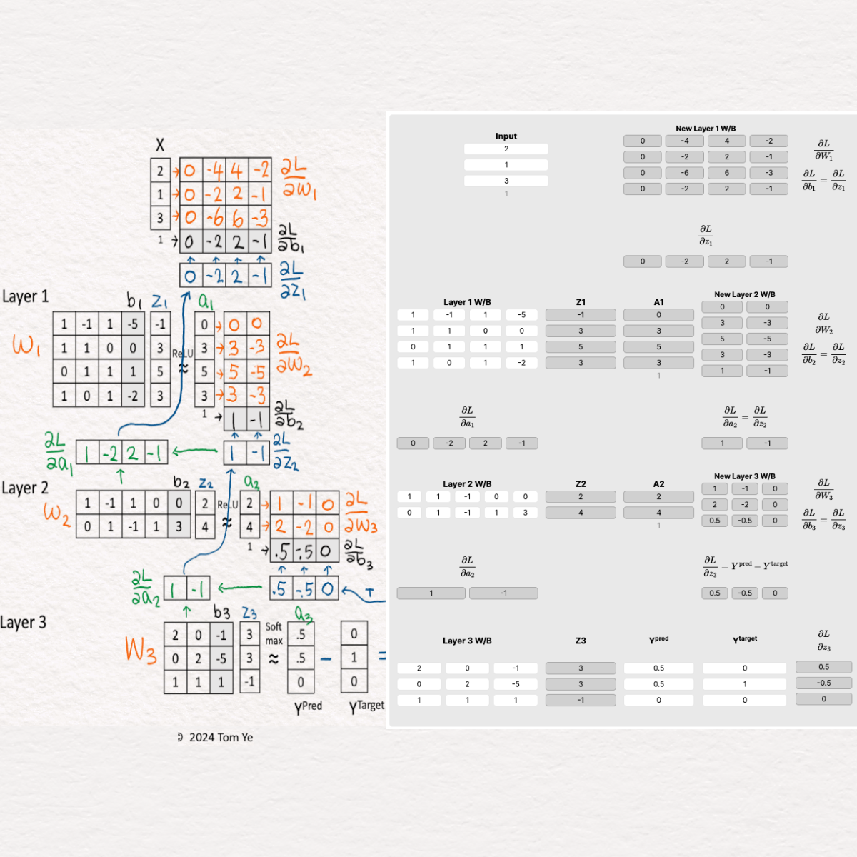
Step 1: Forward Pass

• We start with a MLP network ready to process an input vector X. For simplicity, let’s say the network makes the following predictions: Y^pred = [0.5, 0.5, 0]. We compare these predictions against the actual labels, or the ground truth, which are Y^target = [0, 1, 0]. Straight away, we notice discrepancies between what’s predicted and what’s expected.

Step 2: Backpropagation Begins

• Now, we prepare the network for the crucial task of learning from its mistakes. This preparation involves setting up variables to hold the calculations critical for adjusting the network’s weights and biases.

Step 3: Layer 3 - Softmax and Cross-Entropy Loss

• At this layer, we directly compute the gradient of the loss with respect to z3 using the equation: Y^pred - Y^target = [0.5, -0.5, 0]. This calculation is streamlined thanks to the combination of Softmax and Cross-Entropy Loss, showcasing their compatibility in simplifying backpropagation.

Step 4: Layer 3 - Weights and Biases

• Next, we determine how much each weight and bias at this layer contributed to the overall error. This is done by calculating ∂L / ∂W3 and ∂L / ∂b3, involving a multiplication of ∂L / ∂z3 and the activations from the previous layer [a2 | 1].

Step 5: Layer 2 - Activations

• To understand the impact of Layer 2’s activations on the final output, we compute ∂L / ∂a2 by multiplying the gradient from Layer 3 ∂L / ∂z3 by the weights of Layer 3 W3.

Step 6: Layer 2 - RELU

• The RELU function introduces non-linearity, and here we calculate ∂L / ∂z2 by applying RELU’s rule: multiply ∂L / ∂a2 by 1 for positive values and 0 for negatives.

Step 7: Layer 2 - Weights and Biases

• Similar to Layer 3, we find ∂L / ∂W2 and ∂L / ∂b2 by multiplying the gradient of z2 with the activations from Layer 1 [a1 | 1], further dissecting the error’s source.

Step 8: Layer 1 - Activations

• The influence of Layer 1’s activations on subsequent layers is calculated by multiplying ∂L / ∂z2 by Layer 2’s weights W2, resulting in ∂L / ∂a1.

Step 9: Layer 1 - RELU

• Applying RELU again, we determine ∂L / ∂z1 by multiplying ∂L / ∂a1 with 1 for positive values and 0 for negatives, following RELU’s activation principles.

Step 10: Layer 1 - Weights and Biases

• Finally, we calculate ∂L / ∂W1 and ∂L / ∂b1 by multiplying the gradient of z1 by the original input vector X, pinpointing how each input feature influences the prediction error.

Step 11: Gradient Descent

• With all the gradients calculated, we can now update the weights and biases using gradient descent (typically with a learning rate applied). This adjusts the network’s parameters, guiding it towards more accurate predictions.

The synergy between backpropagation and gradient descent is what allows neural networks to learn and adapt. Backpropagation provides the crucial information needed to guide the optimization process, while gradient descent uses that information to efficiently update the network’s parameters. It’s a beautifully integrated system that enables neural networks to tackle increasingly complex problems with remarkable success.

Interactive Code Environment

Original Inspiration

The inspiration for this deep dive came from a series of hands-on exercises shared on LinkedIn by Dr. Tom Yeh. He designed it to break down the complexities of deep learning into manageable, understandable parts, with a particular focus on a seven-layer MLP. By highlighting the power of interactive learning in a neural network, it starts to show how you can see beyond the ‘black box’ and grasp the nuanced mechanisms at play.

Conclusion: Embracing the Complexity, Mastering the Fundamentals

As we’ve explored the intricacies of backpropagation and gradient descent, it’s clear that the learning process of neural networks is a complex and multi-faceted endeavor. From the mathematical nuances of the chain rule to the intricate dance between forward and backward propagation, there is a wealth of depth and sophistication underlying these concepts.

However, the true power of backpropagation and gradient descent lies in their elegant simplicity. At their core, these algorithms are built on the fundamental principles of optimization and calculus, using the gradients of a loss function to guide the network towards its most effective configuration. By understanding these core ideas, we can unlock a deeper appreciation for the inner workings of neural networks and harness their transformative potential.

• Last Post: What is a Multi-Layer Perceptron (MLP)?

LinkedIn Post: Coding by Hand: Backpropagation and Gradient Descent